Integrating deep learning capabilities into embedded systems has become a crucial aspect of modern IoT applications. Although powerful deep learning models can achieve high recognition accuracy, deploying these models on resource-constrained devices poses considerable challenges. This article presents a gesture recognition system based on the ESP32-S3, detailing the entire workflow from model training to deployment on embedded hardware. The complete project implementation and code are available at esp32s3-gesture-dl. By utilizing ESP-DL and incorporating efficient quantization strategies with ESP-PPQ, this study demonstrates the feasibility of achieving gesture recognition on resource-limited devices while maintaining satisfactory accuracy. Additionally, insights and methodologies were inspired by the work described in Espressif’s blog on hand gesture recognition, which significantly influenced the approach taken in this article.
This article provides an overview of the complete development process for a gesture recognition system, encompassing dataset preparation, model training, and deployment.
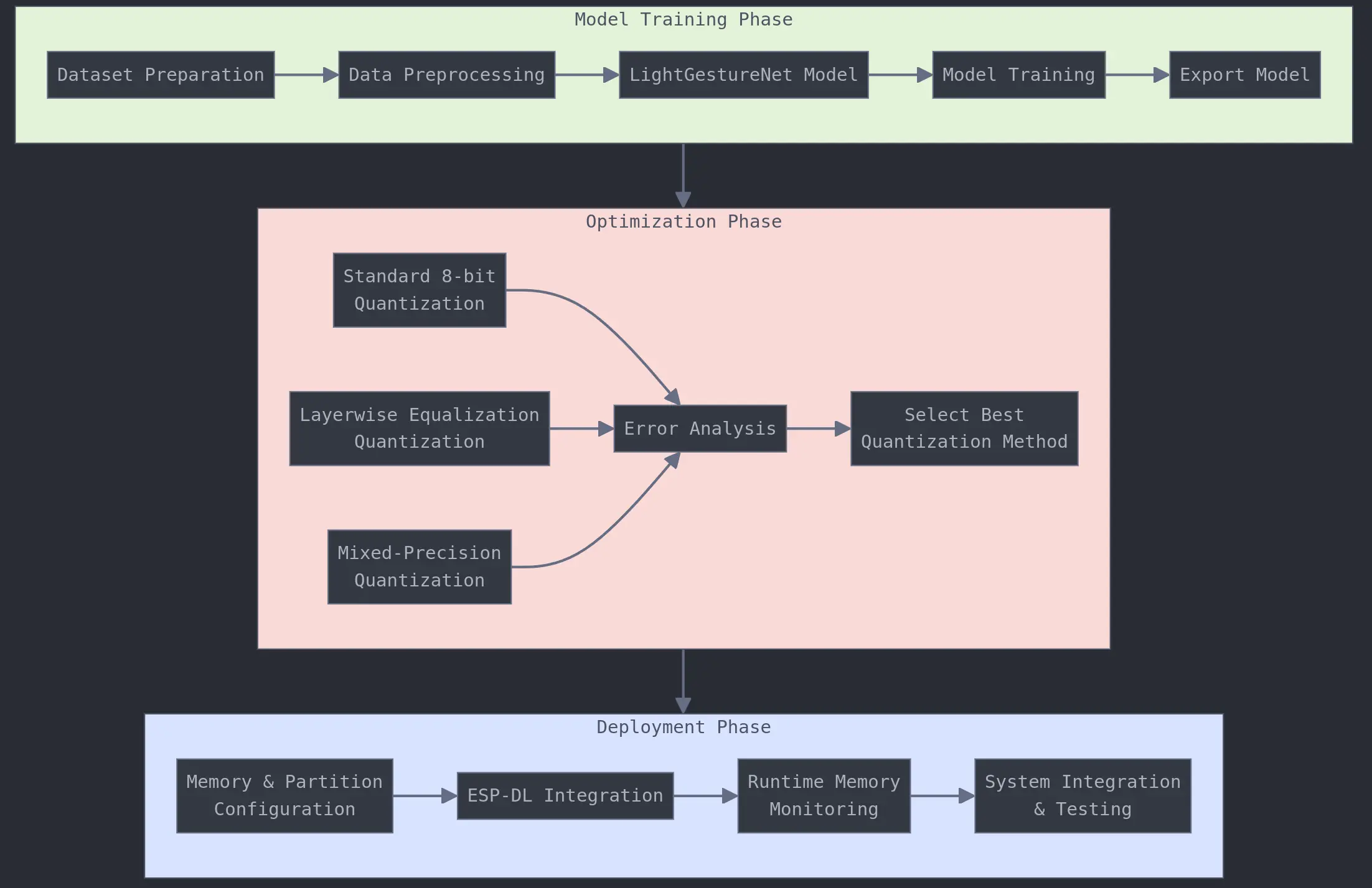
The content is organized into five main sections. The first section, “System Architecture and Configuration,” outlines the overall system architecture and development environment. The second section, “Model Development,” addresses the design of the network architecture and the training strategy. The third section discusses techniques for “Quantization Optimization.” The fourth section focuses on “Resource-Constrained Deployment,” and the final section presents a comprehensive analysis of experimental results.
System Architecture and Configuration#
The gesture recognition system is built upon the ESP32-S3 platform, leveraging its computational capabilities and memory resources for deep learning inference. The system architecture encompasses both hardware and software components, carefully designed to achieve optimal performance within the constraints of embedded deployment.
Development Environment#
The development process requires two distinct Conda environments to handle different stages of the workflow. The primary training environment, designated as ‘dl_env’, manages dataset preprocessing, model training, and basic evaluation tasks. A separate quantization environment, ’esp-dl’, is specifically configured for model quantization, accuracy assessment, and ESP-DL format conversion.
For the deployment phase, ESP-IDF version 5.3.1 is used. The implementation relies on the master branch of ESP-DL and ESP-PPQ for enhanced quantization capabilities. The specific versions used in this implementation can be obtained through:
git clone -b v5.3.1 https://github.com/espressif/esp-idf.git
git clone https://github.com/espressif/esp-dl.git
git clone https://github.com/espressif/esp-ppq.git
For reproducibility purposes, the exact commits used in this implementation are:
- ESP-IDF: c8fc5f643b7a7b0d3b182d3df610844e3dc9bd74
- ESP-DL: ac58ec9c0398e665c9b1d66d3760ac47d1676018
- ESP-PPQ: edfd2d685f88e5b17f773981647172d0ea628ae3
It is important to note that using released versions of ESP-DL (such as idfv4.4 or v1.1) may not yield the same quantization performance as the latest master branch. The system configuration requires careful memory management, particularly in handling the ESP32-S3’s PSRAM. This is configured through the ESP-IDF menuconfig system with specific attention to flash size and SPIRAM settings.
Memory Management#
The system implements a sophisticated memory management strategy to optimize resource utilization. The CMake configuration is structured to properly integrate the ESP-DL library:
cmake_minimum_required(VERSION 3.5)

set(EXTRA_COMPONENT_DIRS
"$ENV{HOME}/esp/esp-dl/esp-dl"
)

include($ENV{IDF_PATH}/tools/cmake/project.cmake)
project(gesture_recognition)
__Note: Ensure that CMake can locate the esp-dl library cloned from GitHub by using relative paths to reference the esp-dl directory.
Component registration is handled through a dedicated CMakeLists.txt configuration:
idf_component_register(
SRCS
"app_main.cpp"
INCLUDE_DIRS
"."
"model"
REQUIRES
esp-dl
)
The memory architecture prioritizes efficient PSRAM utilization, with model weights and input/output tensors strategically allocated to optimize performance. Runtime monitoring of memory usage is implemented through built-in ESP-IDF functions:
size_t free_mem = heap_caps_get_free_size(MALLOC_CAP_SPIRAM);
ESP_LOGI(TAG, "Available PSRAM: %u bytes", free_mem);
This comprehensive system design forms the foundation for subsequent model development and deployment stages, ensuring robust performance within the constraints of embedded hardware. The careful consideration of memory management and environment configuration is crucial for successful deep learning deployment on resource-constrained devices.
LightGestureNet Model Training#
Dataset Preparation and Augmentation#
This implementation processes a gesture recognition dataset through a comprehensive preprocessing pipeline that converts images to 96x96 grayscale format and normalizes pixel values to [0,1]. The core preprocessing functionality handles image loading, grayscale conversion, resizing, and normalization through cv2 operations:
def preprocess_image(image_path):
    img = cv2.imread(image_path)
    gray = cv2.cvtColor(img, cv2.COLOR_BGR2GRAY)
    resized = cv2.resize(gray, TARGET_SIZE)
    normalized = resized.astype('float32') / 255.0
    return normalized
The data collection process implements a systematic mapping between gesture folders and numerical labels, processing all images within the dataset structure. The implementation uses a dictionary-based label mapping system and iterates through the directory hierarchy to build the processed dataset:
gesture_to_label = {
    '01_palm': 0, '02_l': 1, '03_fist': 2, '05_thumb': 3,
    '06_index': 4, '07_ok': 5, '09_c': 6, '10_down': 7
}

def collect_data():
    images, labels = [], []
    for class_dir in [f"{i:02d}" for i in range(10)]:
        for gesture_folder in gesture_folders:
            for img_name in os.listdir(gesture_path):
                processed_img = preprocess_image(img_path)
                images.append(processed_img)
                labels.append(gesture_to_label[gesture_folder])
The processed dataset undergoes a strategic splitting procedure using scikit-learn’s train_test_split function with stratification, creating training (70%), calibration (15%), and test (15%) sets. Each processed image is represented as a float32 array and saved in pickle format for subsequent model development phases. The implementation includes a modular structure for data augmentation, currently implemented as a placeholder, allowing for future extensions of the preprocessing pipeline through additional augmentation techniques.
Model Architecture Overview#
LightGestureNet is designed as a lightweight convolutional neural network for gesture recognition, drawing inspiration from MobileNetV2’s efficient architecture. Here’s a detailed look at the implementation:
class LightGestureNet(nn.Module):
    def __init__(self, num_classes=8):
        super().__init__()

        self.first = nn.Sequential(
            nn.Conv2d(1, 16, 3, 2, 1, bias=False),  # Input: 96x96, Output: 48x48
            nn.BatchNorm2d(16),
            nn.ReLU6(inplace=True)
        )

        self.layers = nn.Sequential(
            InvertedResidual(16, 24, 2, 6),
            InvertedResidual(24, 24, 1, 6),
            InvertedResidual(24, 32, 2, 6),
            InvertedResidual(32, 32, 1, 6)
        )

        self.classifier = nn.Sequential(
            nn.AdaptiveAvgPool2d(1),
            nn.Flatten(),
            nn.Linear(32, num_classes)
        )
The architecture begins with a single input channel for grayscale images and gradually increases the feature depth while reducing spatial dimensions. The initial convolution layer reduces the spatial dimensions by half while increasing the channel count to 16. The network then employs a series of inverted residual blocks, where each block first expands the channels (multiply by 6) for better feature extraction, then performs depthwise convolution, and finally projects back to a smaller channel count. This expand-reduce pattern has been proven effective for maintaining model expressiveness while reducing parameters.
The inverted residual blocks are implemented as follows:
class InvertedResidual(nn.Module):
    def __init__(self, in_c, out_c, stride, expand_ratio):
        super().__init__()
        hidden_dim = in_c * expand_ratio
        self.use_res = stride == 1 and in_c == out_c

        layers = []
        if expand_ratio != 1:
            layers.extend([
                nn.Conv2d(in_c, hidden_dim, 1, bias=False),
                nn.BatchNorm2d(hidden_dim),
                nn.ReLU6(inplace=True)
            ])

        layers.extend([
            nn.Conv2d(hidden_dim, hidden_dim, 3, stride, 1, groups=hidden_dim, bias=False),
            nn.BatchNorm2d(hidden_dim),
            nn.ReLU6(inplace=True),
            # Projection phase: reduce channels back using 1x1 conv
            nn.Conv2d(hidden_dim, out_c, 1, bias=False),
            nn.BatchNorm2d(out_c)
        ])
        self.conv = nn.Sequential(*layers)
The InvertedResidual block implements the expand-reduce pattern with three main components: channel expansion, depthwise convolution, and channel reduction. This design reduces the number of parameters while maintaining model capacity. The use of groups=hidden_dim in the depthwise convolution ensures each channel is processed independently, reducing computational complexity.

Training Configuration and Optimization#
The training configuration implements carefully chosen initialization strategies and optimization parameters:
def weight_init(m):
    if isinstance(m, nn.Conv2d):
        init.kaiming_normal_(m.weight, mode='fan_out', nonlinearity='relu')
        if m.bias is not None:
            init.constant_(m.bias, 0)
    elif isinstance(m, nn.BatchNorm2d):
        init.constant_(m.weight, 1)
        init.constant_(m.bias, 0)
    elif isinstance(m, nn.Linear):
        init.xavier_normal_(m.weight)
        if m.bias is not None:
            init.constant_(m.bias, 0)

model = LightGestureNet().to(device)
criterion = nn.CrossEntropyLoss()
optimizer = optim.Adam(
    model.parameters(),
    lr=0.001,
)
scheduler = optim.lr_scheduler.CosineAnnealingLR(
    optimizer,
    T_max=num_epochs
)
model.apply(weight_init)
Convolutional layers use He initialization, which is particularly suitable for ReLU-based networks as it prevents vanishing gradients in deep networks. BatchNorm layers are initialized to initially perform an identity transformation, allowing the network to learn the optimal normalization parameters during training. The final linear layer uses Xavier initialization, which is suitable for the classification head where the activation function is not ReLU.
The Adam optimizer is chosen for its adaptive learning rate properties, making it robust to the choice of initial learning rate. The cosine annealing learning rate scheduler provides a smooth transition from higher to lower learning rates, helping the model converge to better minima.
Training Process and Monitoring#
The training process incorporates monitoring mechanisms to maintain model performance. Training and validation accuracy thresholds are set at 95–99% and 90–98%, respectively, with a maximum allowable difference to mitigate overfitting. An early stopping mechanism with a patience period of 5 epochs halts training when validation loss plateaus, helping to prevent unnecessary computation and identify issues such as incorrect model output shapes. The best model weights are saved based on validation performance.
Model Export#
The trained model is exported in multiple formats, each serving a specific purpose in the deployment pipeline. The PyTorch native format (.pth) is maintained for continued development and fine-tuning scenarios. The ONNX format is chosen for its cross-platform compatibility and widespread support across different deployment environments, particularly in production settings. The export process implements dynamic batch size support, allowing for flexible inference requirements during deployment.
For mobile deployment scenarios, TensorFlow Lite conversion is implemented with optimizations for mobile environments. Each exported format undergoes a verification process to ensure prediction consistency, maintaining the model’s accuracy across different runtime environments.
Quantization Optimization#
Model quantization serves as a critical bridge between high-precision deep learning models and resource-constrained embedded systems. For the ESP32-S3 platform, three distinct quantization strategies have been developed and implemented, each offering unique advantages for different deployment scenarios.
Quantization Implementations#
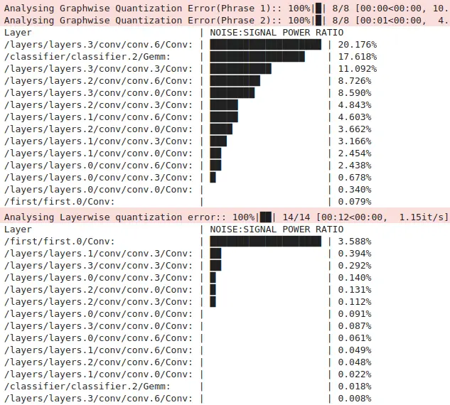
Standard 8-bit Quantization#
The baseline implementation provides straightforward integer quantization while maintaining exceptional model accuracy. This approach represents the most fundamental form of quantization, converting floating-point weights and activations to 8-bit integers. The implementation leverages the PPQ framework’s espdl_quantize_onnx function, which handles the intricate process of determining optimal quantization parameters through calibration. The calibration process takes 50 steps to balance comprehensive parameter estimation and computational efficiency:
graph = espdl_quantize_onnx(
    onnx_import_file=MODEL_PATH,
    espdl_export_file=EXPORT_PATH,
    calib_dataloader=cal_loader,
    calib_steps=50,
    input_shape=[1, 1, 96, 96],
    target="esp32s3",
    num_of_bits=8,
    device="cpu"
)
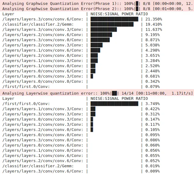
Layerwise Equalization Quantization#
This method solves the common challenge of different weight distributions between network layers by applying equalization techniques. Extensive experiments and parameter adjustments have been conducted to identify the optimal configuration. The current configuration, which achieves the best results, includes the following settings:
setting = QuantizationSettingFactory.espdl_setting()
setting.equalization = True
setting.equalization_setting.opt_level = 2
setting.equalization_setting.iterations = 10
setting.equalization_setting.value_threshold = 0.5
setting.equalization_setting.including_bias = True
setting.equalization_setting.bias_multiplier = 0.5
setting.equalization_setting.including_act = True
setting.equalization_setting.act_multiplier = 0.5
Adjustments across various levels, including opt_level (1 and 2), iterations (1, 2, 5, 10, and higher, where changes beyond 10 became negligible), and value_threshold (0, 0.5, and 2), confirm this configuration as the most effective.
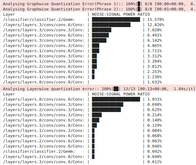
Mixed-Precision Quantization#
The mixed-precision approach represents the most nuanced quantization strategy, enabling precision customization for critical layers while maintaining efficiency in others. To apply 16-bit quantization, select layers with higher Layerwise quantization errors under 8-bit quantization compared to other layers. This implementation recognizes that not all layers in a neural network require the same level of numerical precision. By strategically assigning higher precision to the initial convolutional layer and clipping operation, the approach preserves critical feature extraction capabilities while allowing more aggressive compression in later layers where precision is less crucial:
setting = QuantizationSettingFactory.espdl_setting()
for layer in ["/first/first.0/Conv", "/first/first.2/Clip"]:
    setting.dispatching_table.append(
        layer,
        get_target_platform("esp32s3", 16)
    )
Error Analysis and Performance Validation#
The quantization process requires careful analysis of error patterns and performance metrics to ensure optimal deployment outcomes. The validation framework implements a comprehensive assessment approach that examines both computational efficiency and accuracy retention. This dual focus ensures that the quantized model meets both the resource constraints of the target platform and the accuracy requirements of the application. The testing process utilizes a robust evaluation methodology that processes batches of test data while measuring both inference time and prediction accuracy:
def evaluate_quantized_model(graph, test_loader, y_test):
    executor = TorchExecutor(graph=graph, device='cpu')
    total_time = 0
    correct = 0
    total = 0

    with torch.no_grad():
        for batch in tqdm(test_loader):
            start = time.time()
            outputs = executor.forward(inputs=batch)
            total_time += (time.time() - start)

            _, predicted = torch.max(outputs[0], 1)
            total += batch.size(0)
            correct += (predicted == y_test[total-batch.size(0):total]).sum().item()

    avg_time = (total_time / len(test_loader)) * 1000
    accuracy = (correct / total) * 100
    return avg_time, accuracy
Conclusion#
The evaluation showed that 8-bit quantization and Layerwise Equalization Quantization exhibited varying quantization errors across different layers—some layers demonstrated lower errors with 8-bit quantization, while others performed better with Layerwise Equalization Quantization. However, these differences were minor and did not impact overall performance. Mixed-precision quantization achieved the lowest overall error, but due to the limitations of the esp-ppq version available at the time, which did not support 16-bit quantization on the ESP32-S3, 8-bit quantization was selected for deployment. It is worth noting that the latest version of esp-ppq now supports 16-bit quantization, though this functionality has not yet been tested in this context.
Resource-Constrained Deployment#
The deployment phase of the gesture recognition system on ESP32-S3 requires careful consideration of hardware constraints and system configurations. The implementation focuses on optimal memory utilization and efficient inference execution while maintaining system stability.
Memory and Partition Configuration#
The ESP32-S3’s memory architecture necessitates specific configurations through the ESP-IDF menuconfig system. The following memory settings are crucial for optimal model deployment:
Serial Flasher Configuration
└── Flash Size: 8MB
Component Configuration
└── ESP PSRAM
    ├── Support for external, SPI-connected RAM
    ├── SPI RAM config
    │   ├── SPIRAM_MODE: Octal
    │   ├── SPIRAM_SPEED: 40 MHz
    │   └── Enable SPI RAM during startup
    └── Allow .bss Segment Placement in PSRAM: Enabled
These configurations enable efficient utilization of external RAM for model weight storage and inference operations. The partition table configuration requires customization to accommodate the model data:
Partition Table
└── Partition Table: Custom Partition Table CSV
└── Custom Partition CSV File: partitions.csv
The custom partition layout ensures adequate space allocation for both the application and model data, facilitating efficient model loading during runtime.
Build System Integration#
The project’s CMake configuration integrates the ESP-DL framework and establishes proper component relationships. The build system setup requires careful attention to include paths and dependencies:
idf_component_register(
    SRCS
        "app_main.cpp"
    INCLUDE_DIRS
        "."
        "model"
    REQUIRES
        esp-dl
)
This configuration ensures proper compilation of the application components and correct linking with the ESP-DL framework. The integration of model files and headers follows a systematic approach through the build system.
Runtime memory monitoring#
The implementation employs strategic memory allocation to optimize resource utilization during model inference. Memory monitoring capabilities are integrated into the system to ensure stable operation:
size_t free_mem = heap_caps_get_free_size(MALLOC_CAP_SPIRAM);
ESP_LOGI(TAG, "Available PSRAM: %u bytes", free_mem);
Model weights are stored in PSRAM while keeping critical runtime buffers in internal RAM for optimal performance. The system implements memory monitoring to prevent allocation failures and maintain stable operation during continuous inference.
Serial Communication Configuration#
The deployment setup includes specific serial communication parameters for reliable device interaction:
Component config
└── ESP System Settings
    └── Channel for console output
        └── Default: UART0

Component config
└── ESP System Settings
    └── (115200) UART console baud rate
These settings ensure stable communication during both development and deployment phases. The baud rate selection balances reliable communication with flash programming speed.It has been observed that reinstalling serial port drivers on systems such as Windows 11 and Ubuntu 24.04 can potentially reset the default baud rate and serial port settings. This may lead to issues such as errors in the idf.py monitor tool and the inability to view the corresponding output. In the latest versions of ESP-IDF, the baud rate is automatically set to 115200, mitigating this issue. However, in older versions, such as ESP-IDF 4.4, manual adjustment of the baud rate is necessary to avoid such problems.
Driver Installation and System Integration#
The deployment process requires proper USB driver installation for device communication. The CH340/CH341 driver installation process follows system-specific procedures, ensuring reliable device connectivity.
The deployment process requires proper installation of the USB driver to enable seamless device communication. For the CH340/CH341 driver, system-specific installation procedures must be followed to ensure reliable connectivity.
Experimental Results#
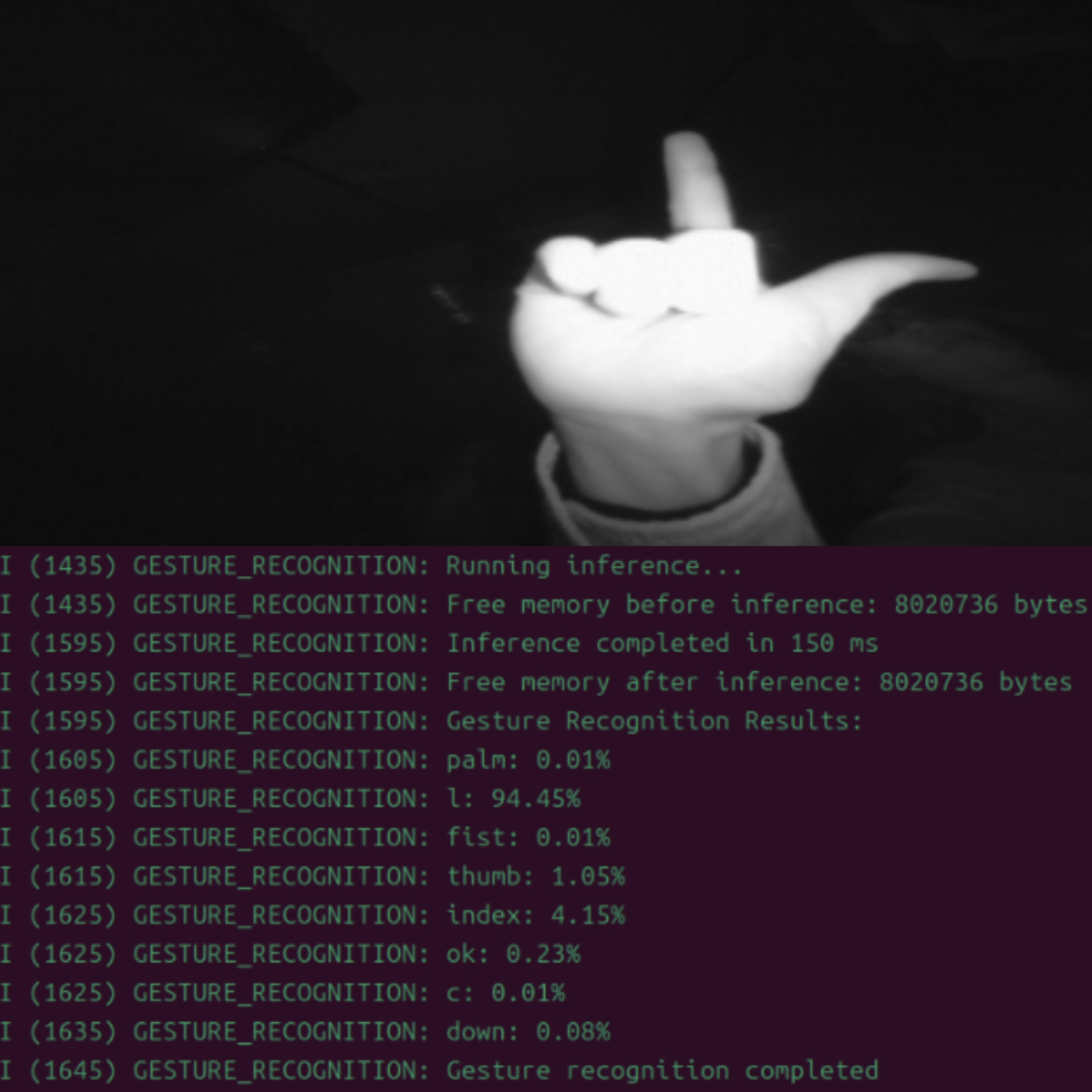
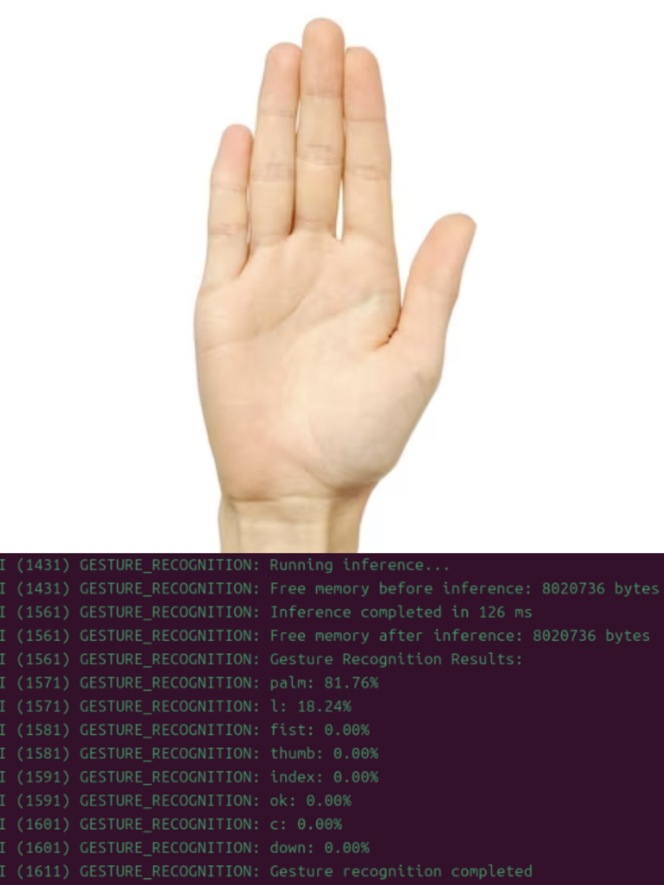
The gesture recognition system on the ESP32-S3 achieves a model loading time of 225 ms and a single inference time of 150 ms, resulting in a total runtime of approximately 375 ms per gesture. A qualitative evaluation was conducted to validate its performance across relevant metrics, including accuracy and model runtime.
The pre-quantization model exhibited high accuracy across eight gesture categories, effectively distinguishing between gestures such as “palm” and “fist.” This floating-point model serves as the baseline for subsequent optimization steps.
After applying INT8 quantization, model size was reduced from 157KB (ONNX format) to 67.2KB (.espdl format) after applying INT8 quantization while maintaining high accuracy. Gesture images from the dataset were accurately recognized, and even images sourced from the Internet performed well after preprocessing.
On the ESP32-S3 platform, the optimized model achieved moderate power consumption and efficient memory utilization, leveraging both internal RAM and PSRAM effectively. These results demonstrate that the adopted optimization strategy is well-suited for deploying advanced gesture recognition systems on resource-constrained hardware platforms.
References#
- ESP official resources
- ESP-DL main repository and documents
- ESP-IDF development framework
- ESP32-S3 Technical Reference Manual
- ESP-IDF Programming Guide
- ESP-PPQ toolchain
- ESP-PPQ project Contains:
- Core API
- Quantizer documentation
- Executor implementation
- Usage guide
- Tutorials and guides
- Datasets